Start date: 01-10-2022
End date: 30-03-2023
Clinical problem
In recent years, over 200 AI products for radiology have come on the market. These products are CE certified, meaning they are approved for clinical use in hospitals. Almost all these products analyze a specific type of radiological image, for example a frontal chest radiograph, and produce a specific output, for example locations of possible pulmonary nodules. Almost all products have been developed using supervised deep learning. A general problem for such products is that they tend to produce nonsense or poor output when an image is input that was not represented in the data that the product was trained on. For example, the chest x-ray nodule detector was very likely not trained with radiographs from children. It won't work at all, of course, on a hand radiograph. It may work poorly on bedside chest x-rays. It could well have been trained only on images from hospitals in Western countries and therefore the product will perform less well on x-rays of middle-age Asian women, a group known to have an increased risk for developing lung cancer. We refer to all this kind of data as out-of-distribution. At the moment, there are no legal requirements for AI products in radiology to systematically perform out-of-distribution detection. We believe legislation enforcing this will be implemented in the next decade and proper out-of-distribution detection will become a requirement for any product so that AI in healthcare will be more robust and reliable.
Solution
The computer vision literature reports many different methods for out-of- distribution detection. We recently tested several approaches and found several to perform poorly on chest radiographs, but one method achieved very promising results: the approach by Dan Hendricks et al. that employs self-supervision, a popular recent trend in deep learning. In this project we would like to use this method, and possibly extend it or compare it to other methods, on a variety of radiological image classification and detection tasks. Our hypothesis is that a generic approach to out-of-distribution detection, trained with self-supervision, will be able to enhance a wide variety of products for AI in radiology.
Data
For this thesis 2 groups of data have been used. The first group contains 3 datasets containing low-dose lung CT scans:
- NLST: 10.183 screening scans
- DLCST: 602 screening scans
- Radboud clinical: 436 clinical scans
For all experiments NLST was used as training data. DLCST was used as a validation set and the Radboud clinical dataset for testing. Since the Radboud clinical contains clinical data it is expected that it also contains OOD data. There are, however, no ID and OOD labels available.
The second group of data contains 2 datasets of x-ray scans:
- Node21: 4882 chest x-ray images
- RadboudXR: 21.576 x-rays.
Node21 was considered ID and used for training. RadboudXR, however, contains a lot of labeled OOD data and was used for testing. Specifically this dataset contains 21,576 samples. 3655 of those are ID and the rest are OOD.
Approach
For this thesis, 4 techniques have been tested for OOD detection.
Rotation and translation
The method proposed by Hendrycks uses RotNet, a network that predicts the rotation angle of an input image, to detect OOD samples. In addition to rotating the input image, the method also applies random translations in both the x and y dimensions, with border reflections. The OOD score is calculated using the softmax probabilities for each of the 36 possible rotation and translation combinations. Summing up the softmax output for the correct class labels gives the final score. Hendrycks showed that the proposed method performs worse on OOD samples than ID samples.
Pre-trained transformer
Large pre-trained transformers can produce high-quality embeddings, which were utilized in this work. Specifically, a transformer pre-trained on ImageNet-21k was employed in conjunction with the Mahalanobis distance. This distance metric was used to compare the embeddings of a group of ID samples to a new, potentially OOD sample. The transformer method can be used in two ways: either as a standalone model with a corresponding classification task and Mahalanobis distance or as the backbone of a self-supervised learning method as described above. In this thesis, both methods were explored.
Relative patch location (RPL)
RPL is a type of predictive self-supervision that involves selecting a random patch and its surrounding patch, and passing them through the same backbone network. The feature outputs are concatenated and sent through a classifier block giving a final output. To avoid picking up trivial patterns such as textures or boundaries that continue between patches, small gaps can be added between the patches. This method can also be extended to work with 3D data, such as CT scans. The size of the 3D cubes can vary depending on the dimensions of the scan, making it useful for scans where the z-dimension tends to be smaller.
Bootstrap your own latent (BYOL)
BYOL is a self-supervised approach that aims to reduce the distance between two representations of the same image with augmented views (positive pairs) while increasing the distance between representations of different images (negative pairs). Unlike previous methods, BYOL prevents model collapse by avoiding gradient flows, which eliminates the need for many negative pairs. This allows for the use of smaller batch sizes, which is particularly important for 3D adaptations. To use BYOL for OOD detection, the cosine similarity between the representations of an augmented input is calculated. With high performance indicating the sample is ID and low performance OOD data.
Results
Node21 & RadboudXR
Below the results can be seen for 8 models and their ability to separate between the RaboudXR ID and RadboudXR OOD data after training on Node21.
| Pediatric | AP | Lateral | Not-CXR | |
|---|---|---|---|---|
| Rot+trans | 0.913 | 0.840 | 0.994 | 0.994 |
| Rot | 0.914 | 0.792 | 0.997 | 0.991 |
| Transformer Mahalanobis | 0.581 | 0.570 | 0.610 | 0.685 |
| Transformer Rot | 0.758 | 0.579 | 0.990 | 0.994 |
| BYOL | 0.700 | 0.601 | 0.774 | 0.680 |
| RPL(ResNet-18, 4 patches) | 0.832 | 0.789 | 0.981 | 0.983 |
| RPL(Resnet-18, 8 patches) | 0.820 | 0.776 | 0.973 | 0.972 |
| RPL(Resnet-50, 4 patches) | 0.901 | 0.799 | 0.986 | 0.990 |
| RPL(Resnet-50, 8 patches) | 0.779 | 0.840 | 0.964 | 0.967 |
As can be seen in the table above the Rot/Rot+trans and RPL method work best. The transformer and BYOL method gave pore results. The transformer method likely gave poor results because it was trained on a different kind of dataset that didn't translate well to the medical domain. The BYOL method was very unstable on an individual sample level. With its results varying a lot based on the kind of augmentations done. For this reason only the Rot/Rot+trans method and RPL method are used in the following experiments.
NLST, DLCST and Radboud clinical
2D
Below the ID scores can be seen after training on the middle axial slice from the NLST training dataset.
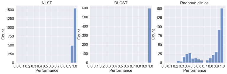
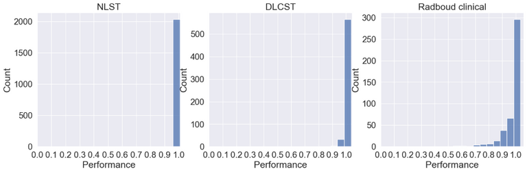
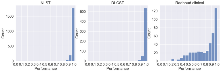
As can be seen the Radboud clinical dataset contains samples with low ID scores that can be potentially flagged as OOD. Doing a visual inspection on these samples with a ID cutoff of 0.7 can be seen below:
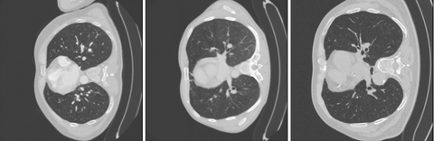
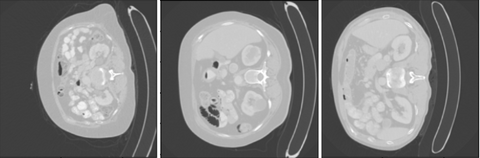
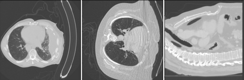
In the 3 images above 3 separates kind of data can be seen. In the top image 3 ID images are shown. In the second image we see images containing the abdomen. The abdomen was not present in the training data and therefore correctly flagged as OOD. The bottom images shows OOD samples that do not contain the abdomen, but were still flagged by the methods.
3D
Where all experiments above worked directly on the whole image or slides a lung nodule classifier might not. For these experiments the nodule malignancy classifier was used. This classifier takes as input nodule blocks of 50x50x50mm around the nodule.
The models are used to categorize the data into 2 groups. This was done by applying a cut-off value at the 90th and 95th percentile of the performance value. Values below the threshold are considered ID and above as potential OOD. By doing this we are able to compare the classifier performance expressed as AUC between the 2 groups. The results of this can be seen in the table below. The Rot+trans method is omitted on nodule level for two reasons. The first one being that it is not possible to predict rotations on a patch level. The method is also not very suitable when dealing with 3D data due to the requirement that all samples in a batch must have the same dimensions. This often poses a challenge, especially in the z-dimension, where it is common for the dimension to vary across samples. As a result, data must be resized to conform to the required dimensions, which may lead to a loss of information. RPL does not have these downsides. It has a flexibility in patch size that is suited for 3D images. The difficulty of the RPL task can also be scaled by reducing the number of patches from 26 to, for instance, 13. Furthermore it has a low memory footprint since it only feeds patches through the network. The time complexity is, however, higher since all possible patches need to be fed through the network to get a final ID score.
| AUC ID 90/10 | AUC OOD 90/10 | AUC ID 95/5 | AUC OOD 95/5 | |
|---|---|---|---|---|
| Rot+trans 2D | 0.86 | 0.90 | 0.86 | 0.95 |
| Rot 3D | 0.86 | 0.89 | 0.87 | 0.84 |
| RPL 2D | 0.87 | 0.78 | 0.86 | 0.92 |
| RPL 3D whole image | 0.86 | 0.94 | 0.86 | 0.96 |
| RPL 3D nodule patch(26) | 0.88 | 0.73 | 0.87 | 0.69 |
| RPL 3D nodule patch(13) | 0.87 | 0.81 | 0.87 | 0.74 |
| RPL 3D nodule patch(7) | 0.86 | 0.94 | 0.86 | 0.92 |
| RPL 3D nodule patch(4) | 0.86 | 0.88 | 0.86 | 0.88 |
As can be seen only the RPL model with 26 and 13 patches are able to predict when the model is going to make mistakes. Highlighting that it is important the input matches the input domain of the classifier. Making the problem easier by using only 7 or 4 patches appears to make the problem too easy allowing the model to still classify patches correctly despite the nodule malignancy classifier failing. A visual inspection on the 5% group for the model with 26 patches can be seen below.
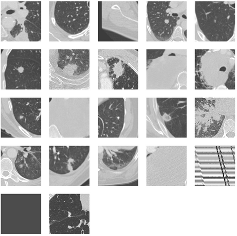
As can be seen in the image above this method was able to detect OOD samples. One of the images detected was corrupted and other nodules flagged are bigger than what was seen during training on NLST.
Cutoff value
In order to utilize such a system in a clinical setting we should be able to detect OOD samples based on statistics and not on a manual cutoff as done above. In the image below all scores are plotted to see if there is a point at which all datasets can be separated. We have also added a pancreas dataset as a control group that the methods should always be able to flag.
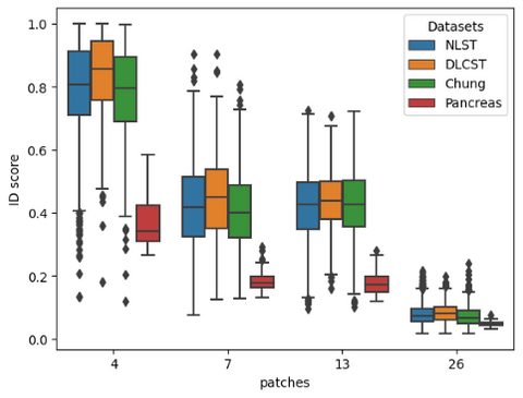
As can be seen in the image above the RPL method is not able to separate all datasets.
Conclusion
We have shown that self-supervision can be used to detect OOD samples. Furthermore we have shown that the state-of-the-art transformer method does not translate well to the medical domain. The results obtained with BYOL where also bad, indicating that more reasearch is needed to see if contrastive method are suitable for OOD detection. There are also still problems with determining a hard cut-off value for clinical usage.